Spectrum Analyzer

Visualizers

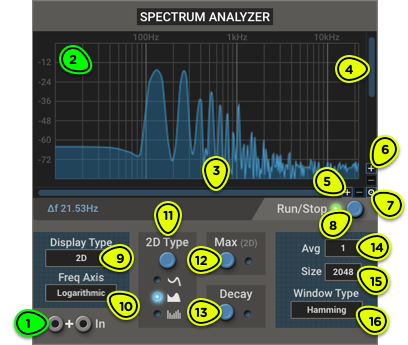
1. Input Signal to be analyzed. If both inputs are connected, their signals will be summed. If no input is connected, the module shows the spectrum of the whole patch.
2. Display Shows the frequency spectrum or the spectrogram of the input signal, depending on the mode.
3. Horizontal Scrollbar Scrolls the frequency axis (spectrum analyzer mode) or adjusts the amplitude color saturation level (spectrogram mode).
4. Horizontal Zoom Sets the zoom level for frequency axis (spectrum analyzer mode) or sets the amplitude range between black and white (spectrogram mode).
5. Vertical Scrollbar Scrolls the amplitude axis (spectrum analyzer mode) or the frequency axis (spectrogram mode).
6. Vertical Zoom Sets the zoom level for the amplitude (spectrum analyzer mode) or frequency (spectrogram mode) axis.
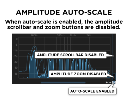
7. Auto-scale Switch Automatically optimizes the amplitude range for the input signal. This disables manual amplitude controls. Click in the display to reset scaling.
8. Run/Stop Button Toggles live spectrum analysis. When stopped, either freezes the last visible frame or waits for the next signal peak to capture a single frame.
9. Display Type Selector Switches between spectrum analyzer mode (2D or 3D), and spectrogram mode.
10. Freq Axis Selector Selects frequency axis scale: logarithmic, linear, or musical notes.
11. 2D Type Selector Selects how data will be represented in 2D mode
12. Max Switch In 2D mode, displays a line connecting the maximum value for all bins. Click on the display to clear the line.
13. Decay Switch Smooths drops in amplitude.
14. Avg Selector Sets how many FFT blocks are averaged, trading quick response for smoother spectra.
15. Size Selector Sets the FFT block size in samples.
16. Window Type Selector Sets the FFT window type.

Overview ⚓︎

The Spectrum Analyzer provides a real-time visual display of its input’s frequency content. It’s a diagnostic and learning tool that can help you:

• balance bass, mid and highs in a patch;
• identify resonances and problematic peaks;
• fine‑tune filters, equalizers, or distortion stages;
• learn about the harmonic series of different oscillators;
• visualize how filters, waveshapers, and modulators affect the spectrum over time.

Usage ⚓︎

When you add the Spectrum Analyzer to a patch, it immediately starts working. If no signal is connected to its inputs, it analyzes the patch output. If a signal is connected to either input, that signal is analyzed instead; if both inputs are connected, their signals are summed before being analyzed.

The module works by splitting its input data in blocks, and obtaining the frequency content of each block with a Fast Fourier Transform (FFT). This data is then processed according to various settings described below and displayed with the selected Display Mode.

The Fast Fourier Transform turns a time-domain signal into a set of so-called frequency bins (or just bins for short). Each bin represents the power of the signal contained in a narrow frequency band.

The module offers many settings to tailor how the signal will be displayed. Refer to the Display Settings and FFT Settings sections below.

If you see something interesting appear on the display and want to spend some time analyzing it, you can manually stop the module with the Run/Stop button. When stopped, the most recent frame remains frozen on the display.

If no signal is present when the analyzer is stopped, it will wait for the next input signal above -60 dB to capture a single frame and freeze it on screen. This lets you capture a snapshot of a transient event.

Display Settings ⚓︎

Display Type ⚓︎

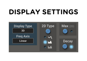
The module offers three display modes in the Display Type menu: 2D, 3D, and Spectrogram.

2D Mode

In 2D mode, the module displays a single block of FFT data.

The 2D Type selector offers three representations:

1. A single line connecting all data points
2. A line with a fill below (nicer to look at, but might render more slowly on some low-end systems)
3. One vertical line for each frequency bin.

2D mode also offers a feature not found in other modes: the crosshair.

Moving the mouse cursor above the curve will show a crosshair at the current amplitude for the nearest frequency bin. Below the display, you will find the frequency, the closest note and the amplitude for the bin at the crosshair position.

3D Mode

3D mode shows the same data as 2D mode, but also shows a trail of older frames previous frames to produce a pseudo-3D waterfall plot.

Spectrogram Mode

Spectrogram mode displays how frequency changes over time, with frequency on the vertical axis and time scrolling from right to left. Each new FFT block is drawn as a vertical “slice” on the right, and older slices move left, creating a scrolling history of the spectrum.

The color intensity represents amplitude, making it easy to spot evolving patterns, transients, and slowly changing tones that might be missed in the other modes.

Freq Axis ⚓︎

The frequency axis can be marked in three ways:

1. Logarithmic
   Logarithmic scale in hertz, matching how the human ear perceives sound. This is the recommended setting.
2. Linear
   Linear scale in hertz. This is the best way to visualize the harmonic series of an oscillator.
3. Notes
   Like logarithmic, but with musical note names instead of hertz. C4 represents the middle C of a piano (many DAWs call it C3). At higher zoom levels, a fine grid shows all notes between octaves. In this mode, we strongly recommend using a window size of 16384 for more precision.

Decay ⚓︎

When the Decay feature is enabled, drops in amplitude are smoothed. This reduces flicker and improves the visibility of transient events.

Zooming and Scrolling ⚓︎

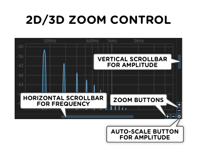
By default, the Spectrum Analyzer shows the spectrum over a wide range of frequency or amplitudes. Depending on your needs, you may want to zoom in on a section of the spectrum.

In 2D and 3D mode, the vertical scrollbar and zoom buttons control the amplitude and the horizontal scrollbar and zoom buttons control the frequency range.

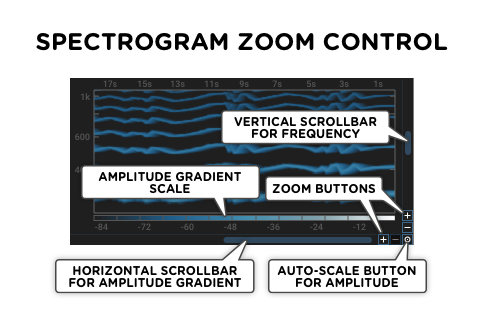
In Spectrogram mode, the vertical scrollbar and zoom buttons control the frequency range, and the horizontal scrollbar and zoom buttons adjust the amplitude gradient.

When a new module is created, it is in auto-scale mode. The amplitude scrollbar and zoom are disabled, and the display automatically adjusts so that the loudest part of the spectrum is visible on screen.

In auto-scale mode, if the signal becomes softer and the amplitude range isn’t satisfactory, you can click anywhere in the display to reset the auto-scaling algorithm and optimize the display for the current spectrum.

FFT Settings ⚓︎

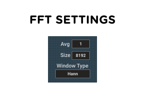
Avg ⚓︎

Avg stands for average. The default is 1, meaning that each update of the display represents only the most recent FFT block.

Averaging multiple blocks will reduce jitter and smooth out transients, giving a better idea of the overall signal loudness at different frequencies.

Size ⚓︎

The Size parameter determines how many samples are processed in each FFT block. A larger block size increases frequency resolution (narrower bins) but also lengthens the time required to acquire a block, which reduces temporal resolution. Conversely, a smaller block size gives quicker updates and better time‑domain tracking at the expense of coarser frequency resolution.

The frequency resolution depends both on the block size and the current sampling rate at which your audio interface is running. The spacing of frequency bins is given by Δf = Fs ÷ N, where Fs is the sampling rate and N is the block size. You will find the value of Δf below the display.

Window Type ⚓︎

After the input signal is split into blocks—but before the FFT is applied—each block can be multiplied by a window function. Different window types will reduce spectral leakage and improve amplitude estimates of the main frequency components, at the cost of a lower frequency resolution.

The four windowing options are Rectangular, Hamming, Hann, and Blackman.

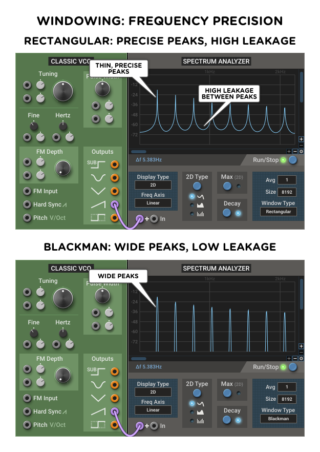
Since an image is worth a thousand words, let’s take a look at how the two opposite window types—rectangular and blackman—handle showing the spectrum of a sawtooth wave.

The following image shows how the rectangular window has thinner, more precise peaks, but more spectral leakage (wide skirts between the peaks). The Blackman window has wider, less precise lobes for the frequency peaks, but exhibits very little leakage between them.

Thanks to its wider lobes, the Blackman window has another advantage: better amplitude precision, as seen in this image:

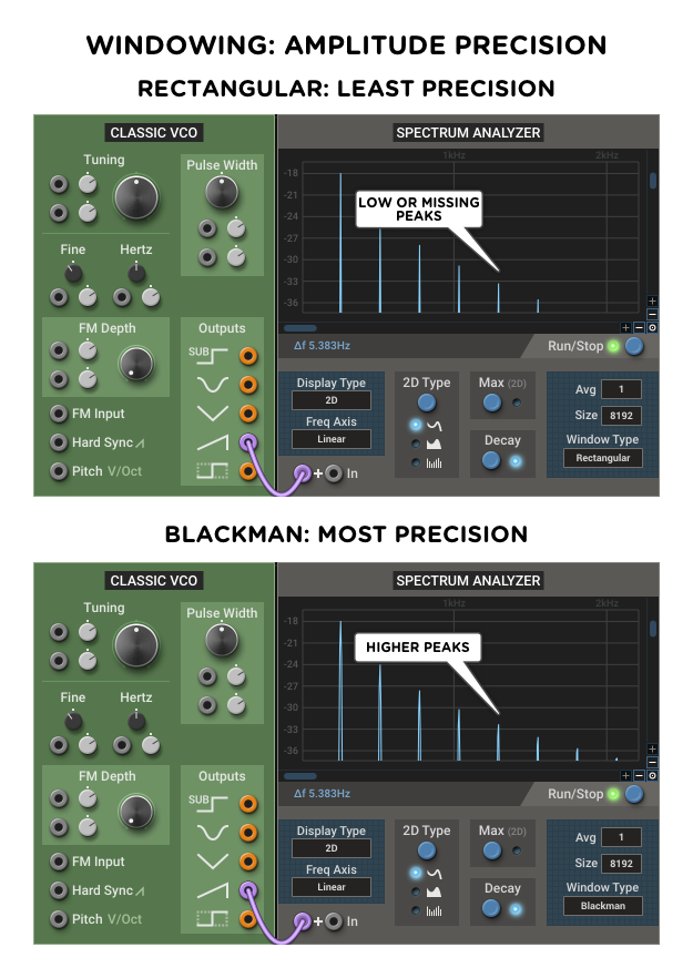
The other two window types are compromises between Rectangular and Blackman: Hamming is closer to Rectangular, and Hann is closer to Blackman.